Paper
Saatchi, Y. and Wilson, A.G., 2017. Bayesian GAN. In Advances in neural information processing systems (pp. 3622-3631).
Vancouver
https://papers.nips.cc/paper/6953-bayesian-gan.pdf
Members of the Group:
- Vincent Casser, vcasser@g.harvard.edu
- Camilo Fosco, cfosco@g.harvard.edu
- Justin Lee, justin_s_lee@g.harvard.edu
- Spandan Madan, spandan_madan@g.harvard.edu
Short Summary
This paper introduces a new formulation for GANs that applies Bayesian techniques, and outperforms some of the current state-of-the-art approaches. It is a true generalization in that we can recover the original GAN formulation given a specific choice of parameters, but authors also show that this formulation allows to sample from a family of generator and discriminators which avoids mode collapse. Posteriors on the parameters of the generator and the disciminator are defined mathematically as a marginalization over the noise inputs. An algorithm is presented to sample from the posterior distributions defining generators and discriminators, using SGHMC and MC.
We will first explain the intuition behind the paper, describe the most important mathematical underpinnings and apply the algorithm to a new, simple problem. Finally, we extend the model on a new, unreleased dataset and show how it performs in comparison to other state of the art methods.
Github
The code and auxiliary notebooks for this tutorial can be found at github.com/jsylee/bayesgan_207 .
This tutorial is best viewed as a jupyter notebook.
TABLE OF CONTENTS
- Introduction to GANs
- Bayesian GAN
- Implementation
- Conclusion
1. Introduction to Generative Adversarial Networks (GANs)
1.1 Overview of the Generative Adversarial Network setup
Generative Adversarial Networks [Goodfellow et al. 2014] are deep neural network architectures consisting of two components: a generator and a discriminator. They are set up to compete against each other (hence the term adversarial), with the following goal. Given some unlabeled input data:
- the generator G tries to generate truly new samples from the input data distribution, therefore implicitly trying to approximate the true data distribution as best as possible
- the discriminator D tries to determine as best as possible if any input was part of the real input data or was generated by the generator G.
Therefore, generator G is trying to fool discriminator D by producing suitable samples, while D is trying to become better at identifiying the artificially generated data. By providing feedback on each other's outputs, the generator and discriminator incrementally improve on their respective tasks.
Of course, the idea of generative and discriminative models is nothing new: given a classification problem, we can generally think about discriminative models (not necessarily discriminators) as approximating $P(y|x)$ for input features $x$ and output label $y$, and generative models as approximating the opposite: $P(x|y)$. [Goodfellow et al.] were the first to draw on that idea and incorporate it in both a competitive formulation (G and D are trying to maximimze and minimize, respectively, a similar loss) and a deep learning setting. In addition, Goodfellow's discriminator doesn't utilize any original labelings $y$ of input data $x$ (in fact, the data doesn't need to be labeled at all), but rather, it determines a new binary label: "real" or "fake". Goodfellow managed to leverage the impressive advances achieved by deep learning methods to tackle this problem on an unprecedented scale.
In principle, any neural network can be seen as simply a non-linear space transformation. Prior to the development of GANs, tasks such as image generation required hand-crafting of loss functions due to the high dimensionality of images; it makes little sense to compare two images using conventional loss functions like the $L_2$ norm. GANs provide a principled way to learn the loss function (indeed, the Discriminator can be seen as a trainable loss function) instead. This is one important reason why most GAN papers look at image-to-image translation, even though the original paper provides a general framework for learning probability distributions.
1.2 A loss function perspective to GANs: A motivation for their need
Most machine learning pipelines can be broadly broken down into the following structure:
- Finding the the right representation for the input data,
- Defining a loss function which is a good metric for estimating how bad the currently learned function performs
- Setting up an optimization which traverses the space of the functions possibly spanned by the model such that the well represented input gets mapped to a point in the output space that minimizes the given metric.
Before deep nets, representation engineering was one of the biggest problems to solve in machine learning, and it required a lot of handwork. For example, in classical computer vision, algorithms such as SIFT, GFTT, and GIST are mostly built on hand-engineered features. Deep Learning addressed this (Point 1). The first few layers of a deep neural network learn a representation for the input data, while the last layer is used for the actual classification. Point 3 above, i.e. optimization, seems to be addressed to a satisfactory degree by stochastic gradient descent. While there are no proofs of this and it is an active area of research, it is generally accepted that existing methods do fine. This leaves only Point 2, i.e. finding the appropriate loss function.
As briefly mentioned in section 1.1, state-of-the-art computer vision required handcrafted loss function for many decades. As such, tasks such as colorization, style transfer, and other complex undertakings could be solved through such custom loss functions with significant effort, but the scope of applicability for such functions was narrow due to their specificity. The natural question to ask is then: is there a way to systematically approximate the right loss function, given an objective and data? This is what generative adversarial networks accomplish. The Discriminator effectively acts like a loss function for the Generator. This extends to the general case: in principle, if we can cast a problem so that it fits the "generator" and "discriminator" setup, we have a method to learn both the input representation, and the loss metric in the output space. This leaves only finding the right optimization technique - for the curious, we reference some recent work on learning: https://arxiv.org/abs/1606.01885.
1.3 Typical Application of GANs: Image generation
One common application of GANs is related to images. We will subsequently describe more concretely how GANs work on the example of image generation.
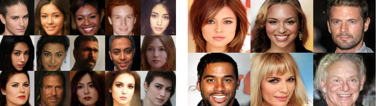
Since the original work by [Goodfellow et al. 2014], the photo-realism of images generated by GANs has improved substantially. With increasingly sophisticated methods for improving the complex training method of GANs, some results are so photo-realistic that they do not noticeably differ from real images even to the human eye. Some state-of-the-art results for face generation are shown in the figure below. However, rather than introducing more advanced methods, we will focus here on the basic method of training.
Training
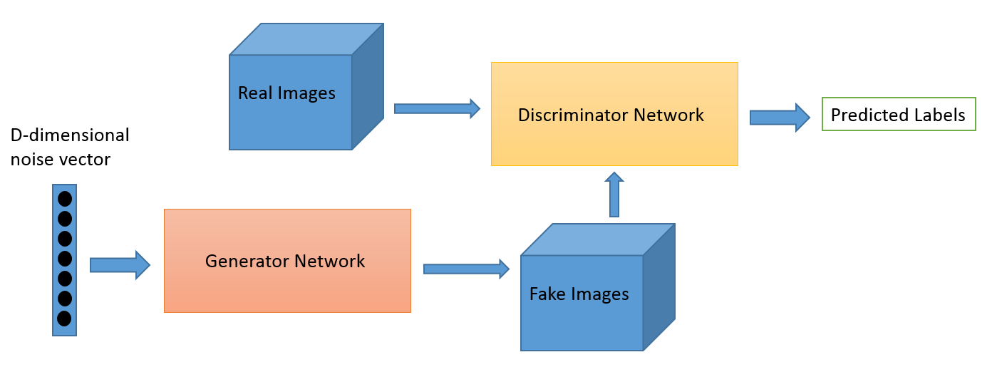
The basic training process of a GAN is an iterative process: we start with the generator G and discriminator D being either randomly initialized or pre-trained neural networks, with the generator taking in some $d$-dimensional noise vector and outputting an image, and the discriminator taking in an image, and outputting a classification score of the input being "original", i.e. true data. We then proceed to train following this process repeatedly:
- The generator G takes in random numbers and returns images. Images are passed into the discriminator D, which provides feedback and whose weights are held steady for the duration of this phase. The generator is trained such that it increases the classification score of the discriminator, trying to make its generated images more realistic and fool the discriminator.
- This generated images are fed into the discriminator alongside a stream of images taken from the actual dataset. That is, while the generator is held steady, the discriminator is trained on recognizing the fakes and originals as such.
The above process can easily be formalized in mathematical terms. G and D can be seen as game agents following a two-player minimax game, as described in classic game theory:
$$\min_{G}\max_{D}V(D,G)=\underbrace{\mathbb{E}_{x\sim p_{data}}[\log{D(x)}]}_\text{$s_1$: true given data}+\underbrace{\mathbb{E}_{z\sim p_z(z)}[\log{(1-D(G(z)))}]}_\text{$s_2$: generated fake data}$$In the above equation, $D(x)$ and $1 - D(G(z))$ represent, respectively, the probability that the discriminator D categorizes true images $x$ and generated or "faked" images $G(z)$ correctly. In simple terms, G tries to minimize the above expression by maximizing $D(G(z))$, consequently minimizing the second term in the sum $s_2$. Since G cannot directly influence the discriminator $D$, it instead tries to model the discriminator's input $G(z)$ so as to fool it. On the other hand, D tries to maximize the expression by increasing $s_1$, correctly classifying the true data as authentic, while simultaneously driving $D(G(z))$ down to zero, causing $s_2$ to vanish as it converges to $\log(1)=0$.
A closer look at the intuition behind the math.
In a GAN we assume that the input data are data points being sampled from a distribution as follows:
Data = $D = \{x_i: x^i \sim p_{data}(x_i)\} $
The goal is to recover an approximation of the distribution so that we can sample from it. For example, if we have a dataset of faces and want to do face generation, then we need to learn the underlying distribution of the face data we have; sampling from this distribution will almost certainly recover a unique face image (due to the distribution being continuous) for each sample.
As it is hard to start with a inductive bias which would fit such a complicated distribution, we usually use as input random noise, which puts no assumptions (i.e. no inductive bias) on the distribution we are trying to sample from.
The hope is that once we are done training, we will have learned a transformation which takes in a random noise vector and transforms it into a sample from the distribution we want: that of faces.
1.4 Common problems
Training a GAN can be tricky and the process unstable, requiring manual intervention and careful parameter tuning. The most common problems include:
Imbalance - one element of the GAN overpowering the other:
If D becomes too adept at separating real images from fakes, it will be so decisive that it returns values extremely close to $0$ or $1$, respectively, such that G has trouble reading the gradient and adjusting its parameters. On the other hand, if G becomes too good, it will continuously exploit weaknesses of the discriminator. The respective learning rates of the networks have to be carefully balanced to tackle this.
Mode-collapse:
If the generator G finds some convenient way to fool D, it can overly exploit this and "overfit" to a specific part of the distribution by transforming most random inputs $z$ into very similar outputs, coming from the same part of the underlying data distribution. We will then have a generator that does not correctly approximate the distribution of the data, but has instead "collapsed" to one of its modes. The resulting generated data will exhibit very poor diversity, limiting the usefulness of the GAN. This can partly be addressed by unbalancing G and D training updates, by anticipating counterplay (the generator learns to fool future versions of the discriminator), or by directly encouraging diversity in samples (feature matching), among others. One of the greatest contribution of the paper we will present here, Bayesian GAN [Saatchi et al. 2017] is a fully Bayesian approach to solve this issue.
For more information on mode collapse, we encourage the reader to visit the following blog post: http://aiden.nibali.org/blog/2017-01-18-mode-collapse-gans/
2. Bayesian GAN
2.1 Why Bayesian Gan?
Recently, there has been quite some work in trying to address the problem of mode collapse, to stabilize GAN training. [Saatchi et al. 2017] propose multiple approaches to improve training and avoid mode collapse. There has also been a lot of research along the lines of improving loss functions, for example, using Wasserstein loss instead of the usual Jensen-Shannon. These methods are very much like regularizing the network to stabilize the optimization. However, there still is no principled approach to do this regularization apart from hand crafted loss functions like Wasserstein.
This paper tackles the regularization process in a principled approach by going Bayesian. As opposed to learning one generator and one discriminator, it learns distributions over possible neural networks in a Bayesian fashion. More precisely, the Bayesian GAN approximates a full distribution over the parameters of the generator and discriminator. But the natural question to ask is, why does this help address mode collapse?
By learning a distribution over parameters, we are essentially learning a distribution of generators. Obviously, this is able to sample from a wider array of datapoints. Suppose we are trying to generate faces - each GAN may sample from a somewhat different distribution of faces. For example, one GAN may be more skewed to sample female faces, while another more skewed to sample male faces. This leads to results with more diversity.
2.2 So what is it exactly?
The Bayesian GAN is a practical Bayesian generalization of the traditional GAN. The idea is to approximate a posterior distribution on the parameters of the generator ($p(\theta_g|D)$) and discriminator ($p(\theta_d|D)$) and use the full distribution to generate data instead of a pointwise estimation. This allows to generate more diverse samples, avoid mode collapse and better represent the underlying distribution. The authors explain that the Bayesian GAN approach presents positive results without any standard interventions such as minibatch discrimination or feature matching. They achieve their results by marginalizing the posterior over the weights of the generator and discriminator using Stochastic Gradient Hamiltonian Monte Carlo. The samples from the posterior define multiple generators that correctly cover the data distribution.
Furthermore, they assert that the inferred data distribution can be used for data-efficient semi-supervised learning. This is a different approach than generating samples: here, we want to train a discriminator to correctly recognize a particular set of classes. Our focus is shifted from the generator to the discriminator. The idea is to get to a good enough point with the generator so that we can simulate data from the original distribution as best as possible, thus having some kind of data augmentation, and using it to improve the classification accuracy of the discriminator. For that, the authors train the discriminator with a loss that both penalizes getting the wrong class and being fooled as well.
Key Insight: This is important, so let's repeat the main idea once more. In a typical GAN, we learn one $\theta_g$ and one $\theta_d$. Here, the goal is to learn a distribution over each of these parameters. By doing so, we are able to recover more diverse samples from the original data distribution, and are able to train this system more reliably with lesser chances of mode collapse.
2.3 Okay, but mathematically, how does it work?
Following the notation of the paper, we would like to estimate the distribution of the data, $p_{data}(x)$, given a dataset $D$ of datapoints $x(i)$ sampled from $p_{data}$. We define a generating system G, called the Generator, that tries to sample from a distribution that approximates this distribution. The role of the generator is to take a sample of white noise z and transform it into a sample from our distribution $p_{data}$. The generator is parametrized by a weight vector $\theta_g$. To train this generator, we build D, the discriminator, parameterized by a corresponding weight vector $\theta_d$. The discriminator, as we have mentioned before, is tasked with outputting a probability that a given data point $x$ comes from the target distribution $p_{data}$.
Up to this point in our work, we described classical GANs. The Saatchi paper extends this concept by proposing to place prior distributions on $\theta_g$ and $\theta_d$. If we do this, we can now build a pipeline similar to a hierarchical model - we use these priors and the likelihood to estimate posteriors on the parameters. In this case, we would obtain generated data by first sampling from the posterior on $\theta_g$, then sampling some noise, and finally using the noise and the sampled parameters to compute the output of the generator. This gives us a sample from $p_{generator}$, which should be close to sampling from $p_{data}$ if the generator is correctly trained.
**Note on abuse of mathematical notation:** Typically, when we say $x \sim p(X)$, we mean that there is a random variable $X$ which is distributed by the pdf (or cdf) p. When we sample from the distribution, $X$ gets instantiated. $x$ is the instantiated value of $X$. It is the same as saying that say, $X$ = number of heads in 5 coin tosses. Here, $X \sim Binomial(5,0.5)$ We can sample from this distribution to obtain that if we tossed 5 coins we would get 3 heads. Then $x$ = 3 is an instatiation of $X$. Here, we are abusing the notation by using the same symbol for $\theta_g$ the random variable which follows the distribution over the generator's weights, and its instantation $\theta_g$, ie both the random variable and it's instantiation use the same symbol. This is a habit popular in many papers, so we follow it here as well.
Mathematically, to get a new set of samples $\bar{x}^{(j)}$, this is what we want to be able to do:
$$\theta_g \sim p(\theta_g|D)$$$$z^{(1)},z^{(2)}....z^{(n)} \sim p(z) \ \ (i.i.d.)$$$$\bar{x}^{(j)} = G(z^{(j)},\theta_g)$$Note the equality in the last equation above. As we have sampled a particular value of $\theta_g$ and $z^{(j)}$, we obtain a single value for $\bar{x}^{(j)}$. This value is a sample from $p_{generator}$, in our case being a generated image.
If we want to be able to do this, we need to find the posteriors. It is important to remember that the generator and discriminator are intertwined - the generator's parameters are directly influenced by the discriminator's, and vice-versa. So to find the posterior for the generator, we need the posterior for the discriminator, which will allow us to sample $\theta_d$ to calculate our likelihood. How do we find the posteriors on the generator and discriminator parameters? The authors propose to iteratively sample from the following distributions:
Distribution 1:
$$p(\theta_g|\textbf{z},\theta_d)\propto \Big(\prod_{i=1}^{n_g}D(G(\textbf{z}^{(i)};\theta_g);\theta_d)\Big)p(\theta_g|\alpha_g)$$Intuition: As we can see, the likelihood term is the product of the output probabilities of the discriminator when the input is fake data. if the discriminator outputs high probabilities, then the posterior will increase in a neighbourhood of the sampled setting of $\theta_g$ (and hence decrease for other settings).
Distribution 2:
$$p(\theta_d | \textbf{z},\textbf{X},\theta_g)\propto \prod_{i=1}^{n_d}D(\textbf{x}^{(i)};\theta_d) \times \prod_{i=1}^{n_g}\Big(1-D(G(\textbf{z}^{(i)};\theta_g);\theta_d)\Big) p(\theta_d|\alpha_d)$$**Intuition:** the first two terms form a discriminative classification likelihood, labelling samples from the actual data versus the generator as belonging to separate classes. And the last term is the prior on $\theta_d$.
$p(\theta_g|\alpha_g)$ and $p(\theta_d|\alpha_d)$ are priors over the parameters of the generator and discriminator, with hyperparameters $\alpha_g$ and $\alpha_d$, respectively. $n_d$ and $n_g$ are the numbers of mini-batch samples for the discriminator and generator.
Intuitively, these equations make sense, as they are the Bayesian expression of the posterior. When we look at the likelihood, we can see that we are encouraging the generator to fool the discriminator - when we fool the discriminator completely, $D(G(\textbf{z}^{(i)};\theta_g);\theta_d) = 1$, and thus the product is maximized. On the other hand, for the discriminator, we have a similar but inverted situation: the likelihood is maximized when $D(G(\textbf{z}^{(i)};\theta_g);\theta_d) = 0$ and $D(\textbf{x}^{(i)};\theta_d) = 1$, which is when the discriminator catches the generator, and when the discriminator correctly recognizes a true sample, respectively.
In most GAN papers, the updates made to the $\theta_g$ and $\theta_d$ estimates are conditional on the chosen set of $z$ vectors in the particular iteration. While this works well in practice, the Bayesian GAN framework goes one step ahead to rule out the bias introduced by the random noise, by marginalizing the noise vector as well. This can be achieved by simple Monte Carlo. As this technique has been discussed in the class, a proof for this has been omitted.
Similarly, $p(\theta_d|\theta_g)$ can also be obtained using simple monte carlo integration marginalizing $z$.
Now, if we observe these equations, we have arrived to a very favorable sitation for Monte Carlo Sampling. It is easy to get noise samples $\textbf{z}$, and both posteriors should be broad over $\textbf{z}$ by construction, since $\textbf{z}$ is used to produce candidate data samples in the generative procedure.
Also, it is interesting to see that if we use flat (i.e. uniform) priors and find the MAP of these posteriors, we end up getting the classical GAN described by Goodfellow et al. The classical GAN can then be called MAP-GAN, or ML-GAN (ML=MAP in the case of flat priors).
Technically, if we sample infinitely from the two given conditional distributions, we obtain samples from the true posterior distribution of $\theta_g$ and $\theta_d$. We are approximating the posterior of the parameters. This is the magic of the BGAN: we are not talking about one specific GAN with fixed parameters, but are instead dealing with a full distribution of generators and discriminators, which themselves characterize distributions of data. We are exploring the full extent of possible GANs given our data.
Another way to interpret the sampling of $\theta_g$ is that we have a collection of generators. When considered together, this "committee" of generators, so to say, can make the discriminator stronger. The multi-modality of the generators also helps prevent GAN collapse. On the other hand, the "committee" of discriminators in turn amplifies the overall adversarial signal, thereby further improving the unsupervised learning process.
Semi-Supervised Learning
So far, we have described the unsupervised learning use of GANs: given just data, learn to reproduce the distribution so that new examples can be generated. However, GANs can also be used for semi-supervised learning. Let's briefly describe what this is and why this is presented in the paper.
Semi-supervised learning can be described as follows: we have a small dataset of labeled points and a larger dataset of unlabelled points, and we want to build a classifier. Semi-supervised learning aims to make the most of that large, unlabelled dataset, even without the labels, to improve the classifier accuracy. This topic is an active research field, and is quite useful - unlabelled data can be found everywhere.
As we mentioned in section 2.2, the paper presents a way to use the BGAN to do pretty good semi-supervised learning. It turns out that the BGAN is suited to this kind of problem, because of the strong coverage of the underlying data distribution.
But first, let's consider for a second why using a simple GAN is in some respects a good idea: we know that if everything works well, we can train a generator to approximate the underlying data accurately. Why not then train the discriminator to not only recognize if the data is fake, but also to predict the correct label? Granted, this seems like a hard task for our poor discriminator, but it is not impossible. Actually, discriminators learn to do it pretty well - given enough training, research shows that we end up with a discriminator that performs better than a simple classifier trained on the small labeled set. The GAN used the unlabeled points to learn the underlying distribution, then generated new examples that were close enough to the real distribution, and than honed the discriminator, which in turn made it become a better classifier. Multiple papers [Kingma & Welling, 2013; Odena, 2016] show that using generative models, and in particular GANs, to leverage large unlabelled datasets leads to more accurate classifiers.
It is clear then that our BGAN should do well in this setting: we are saying that it approximates the underlying distribution better, so it should generate better examples that push the discriminator to become a stronger classifier.
How is it done? Consider a total of n images coming from K classes, such that labels are only known for a small subset. As we said, the goal is to leverage the unlabelled images and the small labelled subset simultaneously to make a good classifier. Any image can either belong to one of the K ground truth classes, or be an image from the generator. Let label 0 correspond to a fake generated image, and 1-K correspond to the K labels on true data. The discriminator only needs to be tweaked such that now $D\left(x(i) = y(i); \theta_D\right)$ gives the probability that sample $x(i)$ belongs to class $y(i)$.
For each sample, we sum over the probability predictions for each class to obtain a tweaked version of the posterior inference formulae for $\theta_d$ and $\theta_g$. This is the only difference in the posterior inference. Here, by summing over probabilities for all possible labels, we are incorporating evidence from both labelled samples (for $y\in(1, ..., K)$), and for unlabelled samples like in the above case (label 0).
Just as before, the posteriors are marginalized over the noise vectors using Monte Carlo.
2.4 Show me some pseudocode.
The main algorithm, implemented below, shows how to compute one iteration of sampling for the Bayesian GAN. The objective is to iteratively repeat these steps to sample the marginalized posterior distributions derived above.
Below, $\alpha$ is the friction term for Stochastic Gradient Hamiltonian Monte Carlo (SGHMC) and $\eta$ is the learning rate. The authors assume that the stochastic gradient discretization noise term $\hat{\beta}$ is dominated by the main friction term (which constrains them to use small step sizes). They draw $J_g$ and $J_d$ simple MC samples for the generator and discriminator respectively, and $M$ SGHMC samples for each simple MC sample.
Here's the algorithm, with some explanatory comments.
Steps:
1. Represent posterior with the previously computed $\{\theta_g^{j,m}\}^{J_g, M}_{j=1,m=1}$, $\{\theta_d^{j,m}\}^{J_d, M}_{j=1,m=1}$.
*We are going to iteratively refine a set of posterior samples with SGD. In the first iteration, we represent our set with random samples, and we will update them as the alogorithm runs.*
2. **For** number of MC iterations $J_g$:
*There are $J_g$ MC iterations: in each one of them, we refine one of our $\theta_g$ samples. This $J_g$ corresponds to the j index used below.*
**a.** sample $J_g$ noise samples { $\textbf{z}^{(1)}, ..., \textbf{z}^{(J_g)}$ } from noise prior $p(\textbf{z})$. Each $\textbf{z}^{(i)}$ has $n_g$ samples.
* Here, we get our noise samples that we will need to compute the MC marginalization of the posterior (the sum over $J_g$ in the parameter update). Note that we use $J_g$ here again, but this time for noise samples, not posterior samples. *
**b.** Update set of samples representing $p(\theta_g|\theta_d)$ by running $M$ SGHMC updates:
$$\theta_g^{j,m} \leftarrow \theta_g^{j,m}+v$$
$$ v \leftarrow (1-\alpha)v + \eta \Big(\sum_{i=1}^{J_g} \sum_{k=1}^{J_d} \frac{\partial log p(\theta_g|\textbf{z}^{(i)}, \theta_d^{k,m})}{\partial\theta_g} \Big) + \textbf{n}$$
* This is the main update step for the $\theta_g samples$. As you can see, we compute one update by looking at the derivative of the log-likelihood (with respect to the weight **vector** $\theta_g$) given our noise samples and our discriminator parameters. The SGD update is akin to the momentum variant of SGD.*
$$\textbf{n} \sim \mathcal{N}(0,2\alpha\eta I)$$
* This noise factor corresponds to the friction parameter of SGHMC. Chen et al. (2014) show that the friction variant of their algorithm introduces this term to minimize the effect of injected noise in the Hamiltonian dynamics.*
**c.** Append $\{\theta_g^{j,m}\}$ to the sample set.
**end for**
3. For number of MC iterations $J_d$:
*We now do the same computations, but for the discriminator parameters. Note that we do $J_d$ iterations here. In the experiments, this parameter is ten times smaller than $J_g$ (1 iteration vs 10).*
**a.** sample $J_d$ noise samples { $\textbf{z}^{(1)}, ..., \textbf{z}^{(J_d)}$ } from noise prior $p(\textbf{z})$. Each $\textbf{z}^{(i)}$ has $n_d$ samples.
**b.** Sample minibatch $n_d$ data samples x.
*One key difference here is that we also have to sample a minibatch of data to compute the log-likelihood.*
**c.** Update set of samples representing $p(\theta_d|\theta_g)$ by running $M$ SGHMC updates:
$$\theta_d^{j,m} \leftarrow \theta_d^{j,m}+v$$
$$ v \leftarrow (1-\alpha)v + \eta \Big(\sum_{i=1}^{J_d} \sum_{k=1}^{J_g} \frac{\partial log p(\theta_d|\textbf{z}^{(i)},x, \theta_d^{k,m})}{\partial\theta_d} \Big) + \textbf{n}$$
$$\textbf{n} \sim \mathcal{N}(0,2\alpha\eta I)$$
**d.** Append $\{\theta_d^{j,m}\}$ to the sample set.
Once we run this algorithm on multiple iterations, we end up with an array of $\theta_d$ and $\theta_g$ samples from their respective posteriors. It is interesting to observe that we get new samples by iterating on previous ones, but we end up with both the old and the new samples on the final array (because we are appending every new iteration). The first samples will be, of course, not as representative as the later ones, so something similar to a burn-in period is needed. In the paper, the authors compute this algorithm for 5000 Iterations, and then take samples every 1000 iterations, which serves this purpose.
2.5 Paper experiments
The experiments proposed in the paper involve 5 datasets: MNIST, CIFAR-10, SVHN, CelebA and a synthetic one, to illustrate robustness over mode collapse. The main comparison approach involves the semi-supervised learning aspect of the problem, where they test their discriminator classification accuracy after training the full GAN with a diminishing number of labeled examples.
In all tests, as we mentioned before, Algorithm 1 is repeated 5000 times, collecting the weights every 1000 iterations. Their values for the internal parameters are:
- $J_g=10$
- $J_d=1$
- $M = 2$
- $n_d=n_g=64$
As can be seen, the values are quite low, as this is a very expensive process to compute (even with shallow G and D networks). They place a $\mathcal{N}(0,10I)$ prior on the generator and discriminator weights, and use a 5-layer deconvolutional GAN as a generator. For the discriminator, they use a 5-layer, 2-class Deep Convolutional GAN (DCGAN) for the unsupervised GAN and a 5-layer, $K + 1$ class DCGAN for a semi-supervised GAN performing classification over K classes.
Synthetic experiment
The synthetic experiment is arguably the most interesting, and the one that better illustrates the robustness to mode collapse of the BGAN. What they do here is generate a very simple dataset (shown in 2D after PCA) with a very clear multi-modal distribution. They then observe samples produced by the generators from the Maximum-likelihood GAN and the Bayesian GAN respectively. They show that with the ML-GAN, there is clear mode collapse: the generated samples all fall in a very particular area of the distribution. With the BGAN, the approximated distribution is much more similar to the original, which shows that the BGAN effectively worked around mode-collapse and produced diverse enough samples that represent the underlying process better.
MNIST experiment
Here, they highlight their impressive performance on the semi-supervised MNIST classification task. They accentuate their results with multiple exclamation marks. Jokes aside, they achieve a very respectable accomplishment: with only 100 labeled training examples, they get to the same classification accuracy (99.3%) of a state of the art supervised method using all 50000 training examples.
On the unsupervised side, they remark that there are some clear differences between the samples they produce and the samples created from a simple DCGAN. Basically, they are showing the expresiveness of their Bayesian formulation: because they are modeling the entire distribution of generator parameters, they can get much more varied MNIST generations simply by sampling new generators from that distribution. They show that the digits created by 6 different generators sampled from the posterior create plausible digits, but from different handwritings. While a DCGAN learns to generate faithful digits with the same style, the sampled generators create different styles (See figure below). The results are, however, not as high-fidelity as in the DCGAN case. The authors explain that this is to be expected: because we are sampling from a distribution over generators, we are not necesarily getting the generator that maximizes the likelihood, which would intuitively give the most high-fidelity results. Instead, the idea here is not to generate photorealistic samples, but instead to generate diverse enough samples so that the full underlying distribution of the data is represented.

To explain perhaps more intuitively, consider a highly bi-modal dataset with modes A and B. We might learn to very accurately reproduce samples from mode A, but never produce points from mode B. A BGAN might produce less faithful datapoints from mode A, but reliably generate datapoints from mode B as well, thus providing a better representation of the underlying distribution.
CIFAR, SVHN, CelebA
These experiments are all very similar. In all cases, they are working with more complex images, and thus more complex underlying distributions. They compare their results on the semi-supervised case, and again, they beat all other methods (Supervised, DCGAN, W-DCGAN, DCGAN-10) on classification accuracy. The unsupervised experiment is not as easy to compare, but it is clear that the diversity of samples coming from the BGAN is superior than the other methods. Each sampled generator also shows a particular style, demonstrating the complementary nature of the different aspects of the distribution learned using a fully probabilistic approach.
References
- [Goodfellow et al. 2014]: Goodfellow, I., Pouget-Abadie, J., Mirza, M., Xu, B., Warde-Farley, D., Ozair, S., Courville, A. and Bengio, Y., 2014. Generative adversarial nets. In Advances in neural information processing systems (pp. 2672-2680).
- [Berthelot et al. 2017]: Berthelot, D., Schumm, T. and Metz, L., 2017. Began: Boundary equilibrium generative adversarial networks. arXiv preprint arXiv:1703.10717.
- [Kerras et al. 2017]: Karras, T., Aila, T., Laine, S. and Lehtinen, J., 2017. Progressive growing of gans for improved quality, stability, and variation. arXiv preprint arXiv:1710.10196.
- [Saatchi et al. 2017]: Saatchi, Y. and Wilson, A.G., 2017. Bayesian GAN. In Advances in neural information processing systems (pp. 3622-3631).
- [Li et al, 2016]: Tgif: A new dataset and benchmark on animated gif description. In Proceedings of the IEEE Conference on Computer Vision and Pattern Recognition (pp. 4641-4650).
- [Kingma & Welling 2014]: Kingma, D.P., Mohamed, S., Rezende, D.J. and Welling, M., 2014. Semi-supervised learning with deep generative models. In Advances in Neural Information Processing Systems (pp. 3581-3589).
- [Odena et al. 2016]: Odena, A., 2016. Semi-supervised learning with generative adversarial networks. arXiv preprint arXiv:1606.01583.
- [Chen et al. 2014]: Chen, T., Fox, E. and Guestrin, C., 2014, January. Stochastic gradient hamiltonian monte carlo. In International Conference on Machine Learning (pp. 1683-1691).
3. Implementation
In this section, we will use the approach described in the paper to train a fairly simple GAN to generate letters. The core implementation was done in pure TensorFlow by the authors and can be found here:
https://github.com/andrewgordonwilson/bayesgan
To follow our tutorial, first clone the github repository. We then recommend running this notebook on a GPU-enabled setup, as the training time for the GAN is otherwise extremely high.
If you directly want to run the GAN training without reproducing all the steps for generating data and modifying the Bayesian GAN framework, feel free to use our included repository and skip to the training section right away.
3.1 O-H Dataset
First, we have to get training data for our GAN to work with. To make this more interesting, we decided to move away from the classic MNIST example, and use our own synthetic data. This is an easy way to generate diverse images in unlimited quantities, and relatively easy to learn by a GAN. Furthermore, we generate a simple but highly bi-modal dataset, where we can easily show how BGAN avoids mode collapse.
import matplotlib.pyplot as plt
import PIL
from PIL import Image, ImageFont, ImageDraw
import numpy as np
import cv2, os, glob, random, string
%matplotlib inline
target_size = 24 #we generate 24x24 images
usr_font = ImageFont.truetype(font='datasets/arial.ttf', size=22)

if not os.path.isdir("datasets/oh_dataset"):
    os.mkdir('datasets/oh_dataset')
We write a simple helper function to generate a random sequence of H's and O's.
def random_charseq(N):
    return ''.join(random.choices(["H", "O"], k=N))
Using the Python Image Library (PIL), we can easily render images with text on them.
def generate_image(word):
    image = Image.new("RGB", (target_size,target_size), (0,0,0))

    d_usr = ImageDraw.Draw(image)
    width, height = usr_font.getsize(word)

    if target_size-width<1 or target_size-height<1: return None # if text does not fit.
    x_rand = np.random.randint(0, max(1, target_size-width))
    y_rand = np.random.randint(0, max(1, target_size-height))
    d_usr = d_usr.text((x_rand,y_rand), word,(255,255,255), font=usr_font)

    image = np.array(image)
    return image[:,:,0]
With the helper functions defined above, let's generate a rendering of single characters (O/H), and plot it.
rw = random_charseq(1)
print('random letter:', rw)
im = generate_image(rw)
if im is not None:
    res = plt.imshow(im, cmap='gray')
else:
    print('the text content was actually out of bounds.')

Now, we can generate variations and store the resulting images in a folder. Below, we generate $N=1000$ images to train our GAN.
N=1000
ct=0
while(ct<N):
    img = generate_image(random_charseq(1))
    if img is None: continue #text actually out of bounds.
    cv2.imwrite('datasets/oh_dataset/' + str(ct) + '.png', img)
    ct+=1
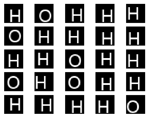
The resulting samples look somewhat like this:
We then proceed to convert the image files into numpy-files (we could have skipped writing the images to disk altogether, if you prefer this).
files = list(sorted(glob.glob(os.path.join('datasets/oh_dataset', '*.png'))))
w_inputs = []
for f in files:
    img = cv2.imread(f, 0)
    img = img.astype(float)/255.
    img = img.reshape((img.shape[0], img.shape[1], 1))
    w_inputs.append(img)
w_inputs = np.array(w_inputs)
print('w_inputs.shape', w_inputs.shape)
np.save('bayesgan_code/W_l.npy', w_inputs)
We also write a vector of dummy outputs.
y_dummy = np.zeros(shape=w_inputs.shape[0], dtype=int)
print('y_dummy.shape', y_dummy.shape)
np.save('bayesgan_code/yw_l.npy', y_dummy)
Now we are left with two files, W_L.npy and yw_l.npy, with the former being the image input of dimension $(N_{samples}, w, h, c)$, and the latter being a vector of dimension $N_{samples}$. In above example, we have $N_{samples}=1000$, $w=h=24$ and $c=1$.
Interfacing with the Bayesian GAN framework
We now need to write an interface for the Bayesian GAN framework to interact with the dataset we created. For this, we follow the example of Saatchi and Wilson by extending bgan_util.py with the following class definition:
class Words:
    def __init__(self):
        self.num_classes = 1
        print('words initializer called')
        self.imgs = np.load('W_l.npy')
        self.test_imgs = np.load('W_l.npy')
        self.labels = np.load('yw_l.npy')
        self.test_labels = np.load('yw_l.npy')

        self.labels = one_hot_encoded(self.labels, 1)        # defined in bgan_util.py
        self.test_labels = one_hot_encoded(self.test_labels, 1)
        self.x_dim = [24,24,1]

        self.dataset_size = self.imgs.shape[0]

    @staticmethod
    def get_batch(batch_size, x, y):
        """Returns a batch from the given arrays.
        """
        idx = np.random.choice(range(x.shape[0]), size=(batch_size,), replace=False)
        return x[idx], y[idx]

    def next_batch(self, batch_size, class_id=None):
        return self.get_batch(batch_size, self.imgs, self.labels)

    def test_batch(self, batch_size):
        return self.get_batch(batch_size, self.test_imgs, self.test_labels)
We change run_bgan.py to import the newly defined Words class.
from bgan_util import Words
And, further down, we make sure to link the words flag to an instance of the class:
elif args.dataset == 'words':
    dataset = Words()
Training
Now that we have prepared the data and framework, we can start the GAN training by running the following cells:
if not os.path.isdir("bayesgan_output"):
    os.mkdir('bayesgan_output')
%run bayesgan_code/run_bgan.py --batch_size 64 --save_weights --data_path ../ --dataset words --num_mcmc 2 --num_gen 1 --num_disc 1 --out_dir bayesgan_output --train_iter 10000 --save_samples --n_save 50
Example results
It is normal for the GAN to take a long time to train. If you do not want to train the GAN from scratch, we have provided some example results below.
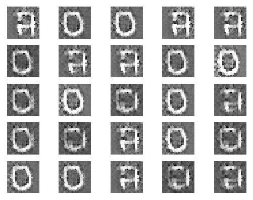
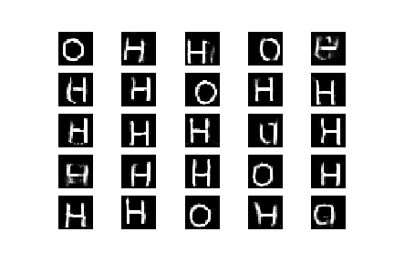
As can be seen, the BGAN correctly approximates this strongly bimodal distribution. After 500 epochs, we start seeing clearly defined Hs and Os, with a healthy diversity in each minibatch. It is interesting to note, however, that during training, certain iterations didn't show as much batch diversity as what we were expecting.
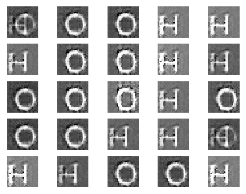
DCGAN: As a baseline, we also observed how a Deep Convolutional GAN performs on this dataset. The code is available in the additional_notebooks folder of our github - as it is not relevant to the BGAN paper itself, we omit it in this notebook. The DCGAN managed to present solid results: in general, we observed high fidelity Os and Hs around epoch 3500. Epochs of DCGAN and BGAN are not directly comparable, but the time taken is - we observed a ten-fold improvement in time taken to get realistic results on the DCGAN. We did see some mode collapse (some batches generated mostly Hs), but in general the diversity is similar to the BGAN. Of course, this is a very simple dataset - the positive aspects of the BGAN appear with more clarity in other situations, as can be seen in section 3.3.
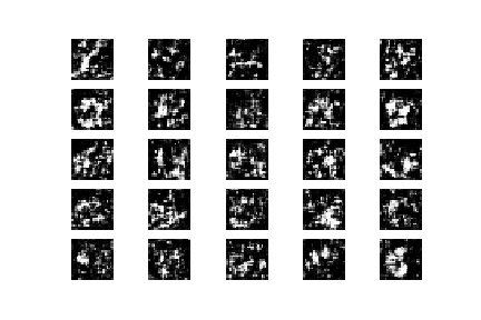
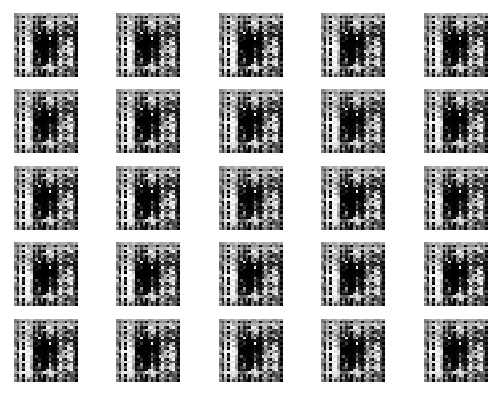
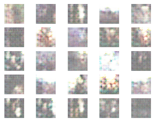
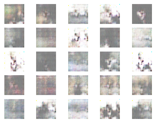
3.2 Results on TGIF
As an additional example, we show the results of the BGAN on a more complex distribution: images from the TGIF dataset [Li et al, 2016]. We want to observe the behavior of the Bayesian GAN when the distribution to approximate incorporates real-world images with multiple backgrounds, color schemes and situations. We are not expecting the network to learn anything close to a credible image, but we are hoping to see a few ordered patterns and some kind evolution from epoch to epoch.
We scraped the TGIF dataset, and extracted center crops for the first frame of all GIFs. The way of feeding this data is exactly analogous to the letter example outlined above. We followed the steps of the tutorial and added an option "tgif" to run_bgan.py, and we created a class TGIF to correctly load the data:
class TGIF:

    def __init__(self):
        self.imgs = np.load('X.npy')
        self.test_imgs = np.load('X.npy')
        self.labels = np.load('y.npy')
        self.test_labels = np.load('y.npy')
        self.labels = one_hot_encoded(self.labels, 1)
        self.test_labels = one_hot_encoded(self.test_labels, 1)
        self.x_dim = [32, 32, 3]
        self.num_classes = 1
        self.dataset_size = self.imgs.shape[0]

    @staticmethod
    def get_batch(batch_size, x, y):
        """Returns a batch from the given arrays.
        """
        idx = np.random.choice(range(x.shape[0]), size=(batch_size,), replace=False)
        return x[idx], y[idx]

    def next_batch(self, batch_size, class_id=None):
        return self.get_batch(batch_size, self.imgs, self.labels)

    def test_batch(self, batch_size):
        return self.get_batch(batch_size, self.test_imgs, self.test_labels)
As you can see in the following results, the images look rather blurry, but some interesting patterns are learned.
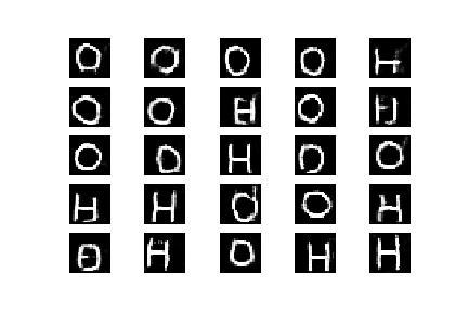
3.3 Results on hand tools dataset
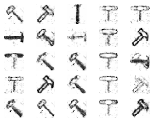
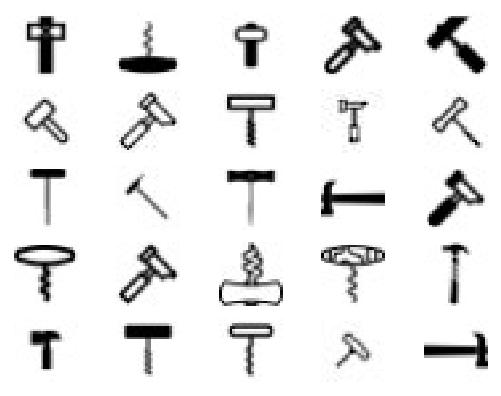
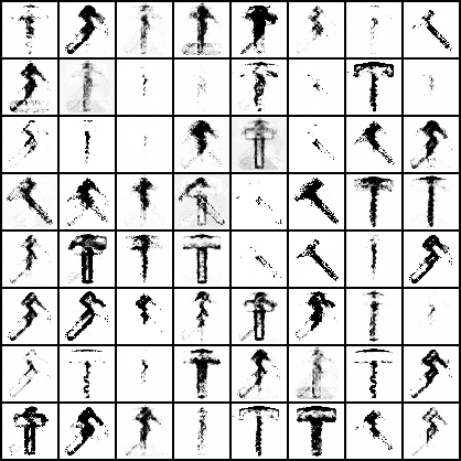
The datasets outlined above still don't quite expose the utility of the BGAN. We decided to collect another dataset of simple objects to further test the BGAN itself. We built a set of grayscale hand tool icons, namely hammers and corkscrews, which is distincticly multi-modal. We observed the behavior of the BGAN when trying to learn this distribution, as well as that of two other generative models: a classic Deep Convolutional GAN and a Variational Autoencoder.
The icon-like images we collected were hand-made by graphic designers, and they often have high diversity, as we can see below. Bayesian GAN is suited to perform well on such a multi modal dataset, so we decided to compare the results to other generative models.

| 
| 
|
Results using Bayesian GAN
As is visible below, Bayesian GAN is able to generate Hammers and corkscrews and it does not suffer from mode collapse. There is a rich diversity in the tools generated.
| 
|
Baseline approaches: DCGAN and Variational Auto Encoders (VAEs)
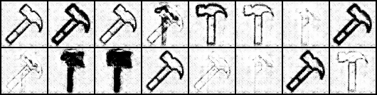
As evident above, DCGAN collapses to only one kind of hammer. This pattern clearly shows the benefit of having a distribution over generators and discriminators in the Bayesian GAN. As the iterations increased for DCGAN, it lost diversity but increased in image quality. The Bayesian GAN did not suffer from this, although it took significantly more iterations to get decent image quality. VAE's were able to handle multiple classes well, but showed poor image quality compared to GANs.
4. Conclusion
Our main takeaway from the BGAN paper is that the Bayesian GAN formulation is useful for generating samples from across an underlying distribution, avoiding the mode collapse that too often plagues GANs. We also realized that although the case the authors make is interesting, the actual practical use of the BGAN is limited. On simple datasets such as OH, the BGAN showed no improvement over a DCGAN, either on diversity of samples or realism of images. On datasets such as the hand-made tool dataset, the results are much better, but the time taken to compute realistic results still limits the usefulness of the BGAN. We do note, however, the positive results achieved on semi-supervised learning - by avoiding mode collapse, a BGAN can be used to generate synthetic, yet realistically diverse training samples from labeled data.
BGANs are exciting, but some technical improvements are still needed to bring this technique to a more general scene. The connection made in Saatchi et al. between GANs and the powerful theoretical toolkit offered by Bayesian inference is respectable, and we foresee that this approach could become much more practical than is currently possible, provided an appropriate computing infrastructure.